How to perform anomaly detection in real-time streaming analytics

Robust Random Cut Forest is a new algorithm for detecting pattern anomalies in real time using both unsupervised learning as well as supervised learning. Know how to detect anomalies real-time in streaming data on the fly.

The key takeaways of the article are:

• Anomalies are data points that do not fit well with the rest of the data
• Anomalies are everywhere, missing them would be dangerous
• Context is important for an anomaly.
• Its relative, what you see as a normal may be an anomaly in a window of events.
• There is no silver bullet to detect and resolve all anomalies.
• Robust Random Cut Forest is a new algorithm for detecting pattern anomalies in real time. Uses both unsupervised learning as well as supervised learning.
• Unsupervised learning defines the normal behaviour and sets the normal parameters and patterns for an algorithm to use that and then detect what is normal and what is not and what is an anomaly.
• Supervised algorithm takes input on what is normal from the Unsupervised algorithm to detect anomalies.

What are anomalies?

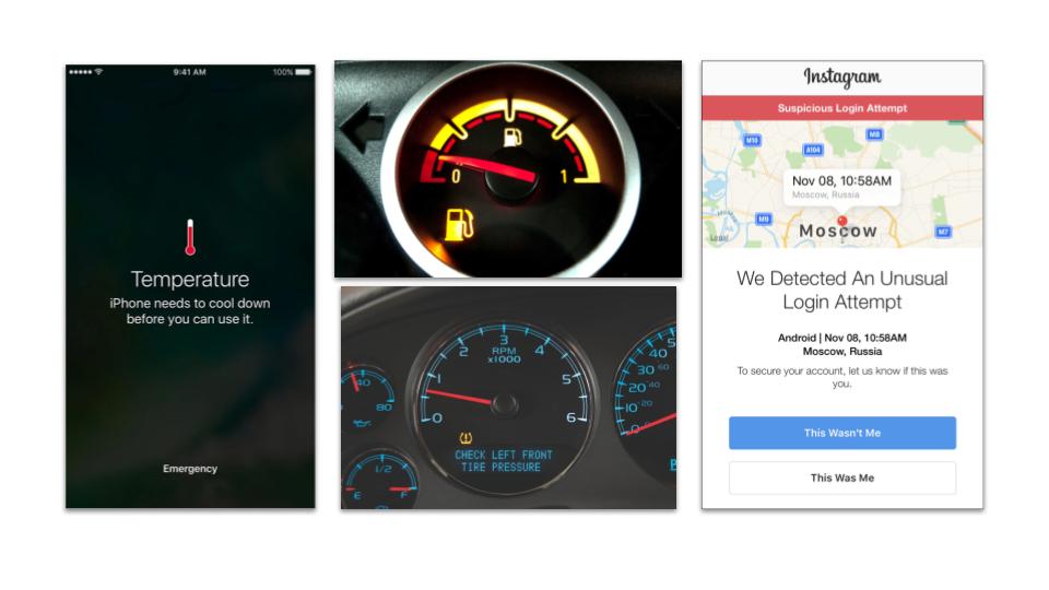
These are the normal alerts or basically the notifications which you see in day to day life, like if you enter into a sauna and take a steam bath, when you come out your iPhone will show that it is too hot to handle. It needs some time to cool down before you can use it. In another example, one fine evening that you are going on a date, when you are driving your car with your date and you look at your fuel meter and notice that you made a blunder. Your fuel tank is almost empty. Or in the morning you have a client meeting and it shows that your front tire has low pressure. It happens, even with Instagram, whenever you change your location and go to a new place or a new country, some applications may give you a notification that an unusual login pattern has been determined. Suddenly you find that you have your credit card in your pocket but you get a notification that you’ve used your credit card in Pittsburgh, and you’re somewhere in Austin on that day. What do all these things have in common? Something is wrong, isn’t it? Something doesn’t fit the pattern. That’s what an anomaly is.

How do you detect anomalies?

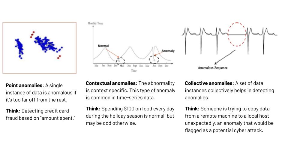
There are many ways, but which one is the right one? You’ve got to know what you’re looking for, and what kind of anomaly you’re looking for. How do you pick the right way? Essentially there are three ways to think about an anomaly. A problem in itself, a single point. Unusually high traffic from an IP address could be a single point anomaly. But, what if there was a dip in the amount of traffic on your website, is your website down? You just had a release and suddenly there’s no traffic on your homepage? That could be more contextual. It could be like for example, on a weekday it is normal to have high usage consumption of electricity on your electric meter, but if the consumption spike happens on a weekend that doesn’t sound right does it? So, what makes sense on a weekday doesn’t make sense on a weekend, that is essentially your context, without which you don’t know if it’s real or if it’s an anomaly. Now thinking about that, look at the third kind. Suddenly things happen in a certain way and there’s a flatline in between. That is an anomaly in a particular sequence, it’s not just one particular point but a sequence of things that happens together that determine any event to be anomalous.

Each of these have specific use cases, some of these make sense to look at in a batch of data. You look at these things and identify one-time standard deviation over two-time standard deviation over. How do you define those points of anomaly? Then, you look at how do you do that when you have training data? With training data even if you have it, it’s hard because anomalies aren’t common. So, somebody who is trying to do something mischievous is going to do the same thing again in the same way, so how do you use that data? How do you make sense of it? Now you can use something like a support vector machine or a Regular Random Forest and try to apply that to get a result, but you’ve got to have the right kind of training data or you can never use those things. How do you do that when you have no such data at your disposal?

How about you try to do that in a more unsupervised manner, but the rate at which you can predict that to happen, it depends upon applying several of those models together and essentially getting those learnings. Let’s think about data in another way, about how data’s value is seen over time. I’m actually trying to define data based on their value, how it accumulates or deteriorates over time. Some amount of data on its own, is not very valuable, but as you accumulate that data and identify trends and patterns in that data, you can actually make sense of it.

But this is way too old fashioned. Are we talking about batch processing in the era of flying cars? Slow and steady wins the race, but how about fast and furious? How about real-time streaming? How about identifying an anomaly or a fraud, or anti- money laundering, when it is actually happening or about to happen and not after it has happened. I think this is the need or demand of the hour and this is what our next topic is, identifying an anomaly in real-time or real-time streaming. This is anomaly detection in real-time streaming, on the fly, in memory, and using Robust Random Cut Forest.

Robust Random Cut Forest

The key features of the alogorithm includes:

• Anomaly detection algorithms are ensemble machine learning models, i.e, models that combine supervised and unsupervised algorithms
• Supervised learning attempts to make a prediction or classification by reverse engineering a set of training data and then applying the learned rules to a new set of data
• Unsupervised learning looks for patterns in data and doesn’t need to be trained to look for any specific pattern
• When used together in an anomaly detection model, unsupervised learning algorithms identify the “normal” pattern for the data, and the outputs from those algorithms train subsequent supervised learning algorithms to classify new data points as either normal or anomalous

How it works?

This is basically an anomaly detection algorithm, it uses both supervised learning as well as unsupervised learning. In unsupervised learning, it reads the data and defines what is normal and then after that when the normal pattern is determined, the supervised learning uses that pattern and identifies what is normal and what is an anomaly.

• As data is fed into the model, it keeps a rolling pool of data points in memory
• Can hold up to 2,147,483,647 data points
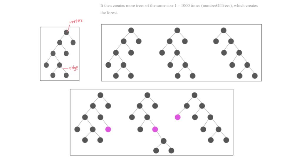
• It uses an ensemble of random forests of trees graphs
• In graph theory, trees are collections of vertices and edges where any two vertices are only connected by one edge
• RRCF starts by constructing a tree of 10 - 1000 vertices (subSample Size) from a random sampling of the “pool” described above
• If we use the defaults for RRCF, that means is constructs a forest of 100 trees that each have 256 data points randomly sampled from a pool of 100,000 data points.
• With the forest planted, we use it to define the normal for a new data point by injecting it into the trees and seeing how much that changes the makeup of the forest.

Robust Random Cut Forest (RRCF) Demo

This is my python code, I am basically using Boto3, connecting to Kinesis, AWS tech, this is the normal heart rate function which gives me the normal data, and the next part is the higher heart rate, which is the anomaly, or anomalous data which I am ingesting in my data. And this is the code which basically 0.01% anomalous data I am ingesting into the stream, and this is where I am connecting it to kinesis. This Python code which I have just shown you is putting the data into input stream, so this is how it works. I am giving my stream a name, how I’ll use it in my code, and then I’m giving only the basic parameters which are required. Then I click on create Kinesis stream.

The stream is created, without schema. I have not mentioned schema right now, what type of data is coming, what are different attributes to it, I have just created the stream. It takes a couple of seconds to create it, and then I move to the next tab, which is data analytics, where I am building my application. So, I clicked on create new application. I am putting the name as demo, as I am a developer, I have a very limited vocabulary. I am running on an SQL engine. Create application, connect to streaming data, so here I am connecting to the existing stream which I created in the first place, and the name is source SQLstream001. Maybe sometimes you’ll get 007. The schema, so this is the place where you can on the fly determine the schema, so I am now triggering my python code, which is going to give the streaming data into kinesis. This is the real-time streaming data, it has two parameters, one is heart-rate and one is type, which is normal or high or low, and I had clicked on discover schema, which basically is on the fly determining the schema, its type, whatever type it is, and you’ll get the result ‘yes, the schema is discovered, voila’, it’s just inform it, and these are the input records. So now, one part of the presentation is kind of complete, where I am able to put the data through the program, not a real-time application, but programmatically I put the real-time data on stream.

Now the next phase is to apply the random robot cut forest algorithm on top of it and try to identify what is anomalous and what is not. The next thing is, I am also demonstrating the part that is particular code, which I have demonstrated in the first part when I created the input stream, I’ve not defined the schema. On the fly, schema is basically defined by looking at the input data stream, so I am using the same stream which I had created, but now I am putting different data to it, and I want to check that it is able to identify the new schema or not. This is the code, so basically it is more related to normal use case detecting fraud, this is a normal transaction, so I am using transaction amount, country code, because a few of the countries are high risk countries where the bank tends to keep an eye on the transactions of those country codes. I’ve basically created three functions; one is a normal transaction with a normal amount from a normal country code. The second is a high amount transaction with maybe a high-risk country, and followed by a low amount transaction from a high-risk country, because a small amount of funds are circulated from multiple accounts and into the wrong hands, so I am keeping track of low value transactions as well as high value transactions. This is the code, it’s quite similar to the previous one, and I am putting the error data or the low transaction or the high transaction to the input stream, and let’s see how it works out.

The next thing I’ll be doing is, I’m going to create a new application in data analytics because the stream is already created. I stopped the previous stream and I’m running my new code, the updated one, so test two. Here is the new transaction, so the new schema is transaction amount, country code, and transaction status which is normal, high or low. I skip the data stream part and I directly move to the data analytics tab, and I am creating a new application. We have multiple options for the previous application but I thought to go for the new application, and that’s what I did. Demo already exist, so demo_1, I’ve placed. Create application, again I’m repeating the same step, connecting to the data stream, I am selecting the previously selected stream, which is example input stream, and now discover schema so I’m basically checking the schema which is the new one or the version 2. Here it is. So, this is the new schema on the fly, same stream which I used, it basically determines the new schema and I’m able to go further.

The next thing I’m doing is, I’m going to the SQL editor, where I can write the SQL code on top of it, so this kinesis provides a SQL interface where you can write SQL transformation on the fly in real-time streaming data. So, I selected the SQL editor, and then just start application, so that they can start charging, three options are there, one is data source, real-time analytics and destination. We just configured the source just now, and the source is source_sql_stream001, and it’s trying to identify the schema and all the records. These are the records, which are generated by my simple python code. A few extra columns have been added for traceability and to uniquely identify those transactions by kinesis. The next thing I am doing is now writing the SQL code where I am using a Robust Random Cut Forest Algorithm. It is very simple, this is the section of code which I have written, this is the temporary stream I am creating for doing transformations, the next thing I am doing is creating an output stream which I want to see by applying some transformations. Let’s say I want to sort it on the basis of some particular column, or do an average or something, I can use this as a destination SQL stream. The most interesting part is applying the algorithm, as this algorithm is an unsupervised algorithm, I am not going to train the algorithm. It just reads the data, reads the input stream, identifies the pattern, what is normal, what is different and what is an anomaly. On the fly, it determines and starts rating the point which is different from the normal pattern. Here it is, I am using it, which is reading the input source stream and then applying the Random Robust Cut Forest Algorithm with explanations. Two versions are available, one is with explanation and the other is without explanation. With explanation we can get the insights of the data or the particular data point.

Just to understand what those parameters mean, it basically helps you understand the number of trees involved in this Random Cut Forest, how many events or elements are in each of those trees, the sub-sample size, how long is that going to be effective in determining what’s valid and what’s not valid. That’s the time decay. The single size helps with how long you keep that for, and directionality helps you determine how to go about doing this, is it going backwards, or forwards.

This is the place where I am applying the algorithm, and this is the destination stream where I am putting it. The last thing which I have to do is save and run SQL. So, it’s saving the SQL and running the SQL. We already saw the source data and now it’s implementing the algorithm and giving you the results. All the data points, the anomaly score is 0.0. So, at the moment it is not discriminating in the data points between what is an anomaly and what is not, it is just internally training itself. It creates a window, analyses those points, understands, trains the model, and then fits the new points and tries to score that particular data point. These are the explanations corresponding to the data point, or each particular point. The destination, the third type, which I have not configured yet, we are basically losing the data. I am not saving it on s3 or any other database. I am just checking the score, and now we are getting the score. So, right now, for a normal data point, we are getting around 0.6, 0.7, 0.9, less than a 1, for the anomaly score, and sometimes when we get any high transaction or low transaction, you will see a different score. For the high one it is 4.2, so now it has started segregating the data and raising an alert by the score, that this is a high data point, its value is 4.2, for low it is showing 2. Something. So, it basically segregates both low as well as high by putting a corresponding score to it. This is it in terms of demo, now the thing is how internally this algorithm works.

What it does is, it creates a tree, it uses Random Forest and classification techniques, it creates the tree based on the data points coming in the window, two vertexes are joined by a single edge, it can hold up to 2,147,483,647 data points and then apply both unsupervised and supervised algorithms and then determine the next data point. If the next data point comes in, how it basically disturbs the forest. So we can configure the number of trees in the forest. This is one of the parameters for our algorithm.

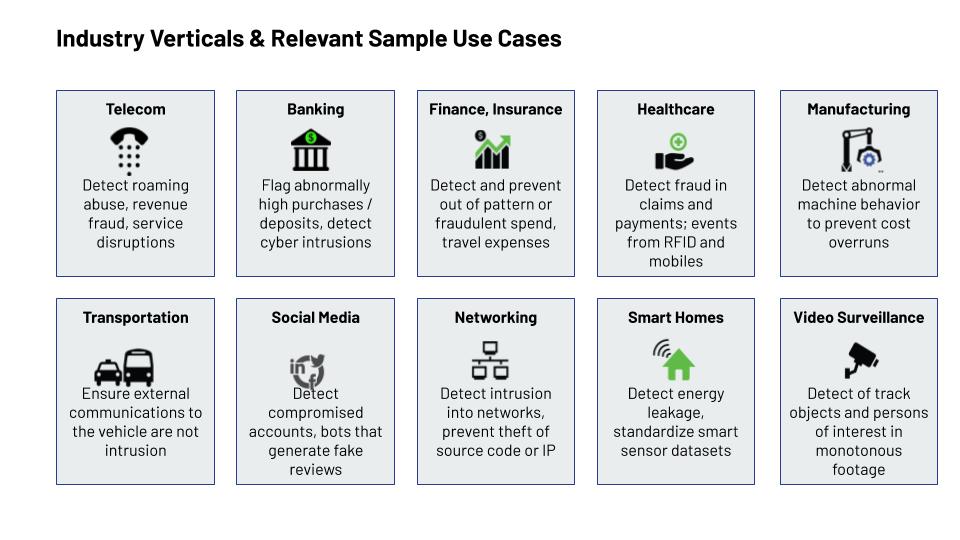
The next thing is, whenever the forest is created in memory in the time, any new data point comes, it calculates how it is deviating from or disturbing the forest. This is how it internally works. These are the different parameters and numbers, the number of trees it creates, or when it gives better performance. This is the function which I used, and corresponding default values for that one. Just like AI or machine learning, the fraud detection or anomaly detection is applicable to all industry, all the verticals, whether it is banking, finance, healthcare or anything, so a few of the use cases which I have mentioned, such as fraud detection or roaming abuse or video surveillance, detecting or tracking the object or a traffic signal, whether somebody is going on the wrong side or not following the lane or something, so it is applicable for every domain.

Just like our use cases, it is applicable for money laundering as well, which I guess banks have started implementing, so a few of the banks are working on it. But most of them, or 99% of the banks in batch mode, not on real-time, so this is basically the first attempt of bringing this on AWS, to my knowledge, implementing real-time streaming analytics. So, the same slide, key takeaways.

We’ve basically established what anomalies are, how do you go about figuring out what the right one to pick is when you have training data and when you don’t. You want to detect the anomalies on the fly. We’ve heard about the concept of digital twins, right? So if somebody else has taken over your digital twin and is spending all your money, you don’t want to know about it several eons later and figure out that ‘oh, it’s all gone. Now I’ve to figure out how to get my money back.’ This sort of talks about the performance in numbers, AWS has also launched a service called SageMaker. These are some of the performance metrics and numbers that we have looked at and how it performs when you have many dimensions. Over there we only looked at a couple of the dimensions, where one is the transaction amount and one was the country, but you can keep adding many more dimensions and look at those things. It sort of shows how the performance was over time, and as you can see, as the number of dimensions increased the performance is a little bit lower, but so has the complexity, right? If you look at the accuracy on the other side, it talks about how the performance was for a hundred million records. The numbers are all based on a synthetic data set, which is a gaussian distribution, with roughly 0.5% anomalies created, so that is the accuracy predictions. Based on that, the client represents how it showed for that 0.5% on the diagram on the right.